Artificial Intelligence A Modern Approach, 3rd Edition
0.1 AI
Artificial intelligence (AI) is the branch of computer science that develops machines and software with intelligence.
0.2 The Turing Test
The Turing Test was designed to provide a satisfactory operational definition of intelligence.
2 people & 1 machine
an interogator: to find out which candidate is the machine or human, only by asking them questions.
If the machine can fool the interrogator 30% of the time, the machine is considered intelligent.
1 Problem Formulation
1.1 Problem Formulation
Problem formulation is the process of deciding what actions and states to consider, given a goal.
1.2 Problem Components
Initial State: the starting state of the problem, defined in a suitable manner.
Actions (Operators): an action or a set of actions that moves the problem from one state to another.
Neighbourhood: The set of all possible states reachable from a given state by applying all legal action(s).
Successor Function: the action(s).
Goal Test: a test applied to a state which returns true if we have reached a state that solves the problem.
Path Cost: how much it costs to take a particular sequence of actions.
A solution to a problem is an action sequence that leads from the initial state to the a goal state.
State Space: the set of all states reachable from the initial state (it forms a directed network or graph), determined by the initial state and the successor function, decides the the complexity of a problem based on its size.
1.3 Problem Representation - Graph
Graph: to model the deeper structure of a problem
Consists:
A set V of nodes
has a unique label for identification
represents possible stages of a problem
A set E of edges
is the connection between two nodes
represents inferences, moves in a game, or other steps in a problem solving process (operator)
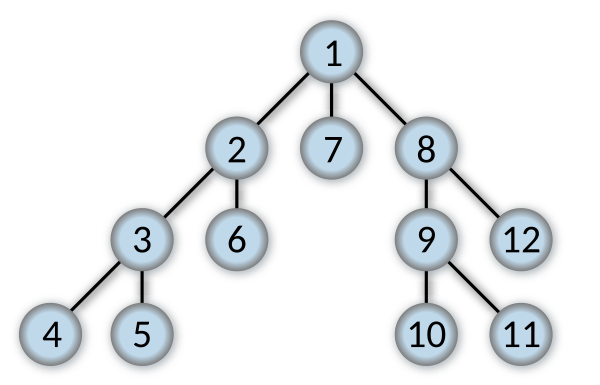
1.4 Search Trees
Tree: a graph that
is connected but becomes disconnected on removing any edge
is connected and acyclic
has precisely one path between any two nodes
Nodes
Root node
Children / parent of nodes
Leaves
Branches
Average branching factor: average number of branches of the nodes in the tree
Depth
of a node: the number of edges (branches) away from the root node
of a tree: the depth of the deepest node
Problem Representation
State: nodes
Initial State: root node
State Space: all nodes in the tree
Neighborhood: the set of all possible states reachable from a given state
Number of neighborhoods: branching factor
Operator(s): branches
How big can a search tree be?
A branching factor b
One goal exists at depth d
bd different branches in the tree
1.5 Properties of Search
Complete Search Methods' properties
If a goal exists then the search will always find it
If no goal exists then the search will eventually finish and be able to say for sure that no goal exists
1.6 Evaluating a search
Completeness: Is the strategy guaranteed to find a solution?
Time Complexity: How long does it take to find a solution?
Space Complexity: How much memory does it take to perform the search?
Optimality: Does the strategy find the optimal solution where there are several solutions?
1.7 Search Tree Issues
Wasteful on space
Difficult to implement
Not always obvious which node to expand next. We may have to search the whole tree looking for the best leaf node. This can obviously be computationally expensive.
2 Search Strategies - Blind Search
2.1 Categories
Uninformed / Blind Search
BFS
DFS
UCS
Informed / Heuristic Search
Greedy Search
A* Search
2.2 Blind Search
2.2.1 Fundamental actions
Expand: ask a node for its children
Test: test a node to see whether it is a goal
2.2.2 General Tree Search
Function General-Search(p, QUEUING-FN) returns a solution or failure.
1
2
3
4
5
6
7
nodes = Make-Queue(Make-Node(Initial-State[p]))
Loop do
	If (nodes is empty) then { return failure }
	node = Remove-Front(nodes)
	If (Goal-Test[p] on State(node) succeeds) then { return node }
	nodes = QUEUING-FN(nodes, Expand(node, Operators[p]))
End
2.2.3 General Graph Search
Function General-Search(p, QUEUING-FN) returns a solution or failure.
1
2
3
4
5
6
7
8
nodes = Make-Queue(Make-Node(Initial-State[p]))
Loop do
    If (nodes is empty) then { return failure }
    node = Remove-Front(nodes)
    If (Goal-Test[p] on State(node) succeeds) then { return node }
    	add the node to the explored set
    nodes = QUEUING-FN(nodes, Expand(node, Operators[p]))
End
2.2.4 Search Strategies
Strategy: picking the order of node expansion
Evaluating strategies
Completeness: does it always find a solution if one exists?
Time complexity: number of nodes generated/expanded
Space complexity: maximum number of nodes in memory
Optimality: does it always find a least-cost solution?
Time and space complexity are measured in terms of
b: maximum branching factor of the search tree
d: depth of the least-cost solution
m: maximum depth of the state space (may be ∞)
2.2.5 Breadth First Search
Method
Expand shallowest unexpanded node
Expand Root Node First
Expand all nodes at level 1 before expanding level 2
…
Expand all nodes at level d before expanding nodes at level d+1
Queuing function: adds nodes to the end of the queue
General-Search(problem, ENQUEUE-AT-END)
Evaluation
Optimal: yes (only if the branch costs are the same)
Complete: yes
Time complexity: O(bd) i.e. the number of leaves
Space complexity O(bd) i.e. the total number of nodes
b: the average branching factor
d: the depth of the search tree
2.2.5 Depth First Search
Method
Expand Root Node First
Explore one branch before exploring another branch
Queuing function: adds nodes to the front of the queue
Function DFS(problem) returns a solution or failure
Search the queue and remove the node of smallest cost
Function UCS(problem) returns a solution or failure
Return General-Search(problem, ENQUEUE-BY-COST)
Evaluation
Optimal: yes (even branch costs are different)
Complete: yes
Time complexity: O(bd) i.e. the number of leaves
Space complexity O(bd) i.e. the total number of nodes
VS. BFS
UCS = BFS (when all branches have the same cost (in the worst case)
UCS is usually better than BFS
https://www.youtube.com/watch?v=dRMvK76xQJI
3 Search Strategies - Heuristics
3.1 Several AI Methods
Heuristics
Fuzzy Logic
Bayes reasoning
Game Theory
Evolutionary Computation
Evolutionary Game Theory
3.2 Definition of Heuristics
A heuristic is any approach to problem solving, learning, or discovery that employs a practical method not guaranteed to be optimal or perfect, but sufficient for the immediate goals. Where finding an optimal solution is impossible or impractical, heuristic methods can be used to speed up the process of finding a satisfactory solution.
3.3 Types of Solutions
A solution to an optimization problem specifies the values of the decision variables, and therefore also the value of the objective function.
A feasible solution satisfies all constraints.
An optimal solution is feasible and provides the best objective function value.
A near-optimal solution is feasible and provides a superior objective function value, but not necessarily the best.
3.4 Continuous & Combinatorial
Continuous: optimization problems that has an infinite number of feasible solutions
Continuous problem generally maximize or minimize a function of continuous variables such as min 4x + 5y where x and y are real numbers
Combinatorial: optimization problems that has a finite number of feasible solutions
Combinatorial problems generally maximize or minimize a function of discrete variables such as min 4x + 5y where x and y are countable items (e.g. integer only)
3.5 Constraints
Hard Constraints: must be satisfied
Soft Constraints: desirable to satisfy
Explicit Constraints: stated in the problem
Implicit Constraints: obvious to the problem
3.6 Search Basics
Search: the term used for constructing/improving solutions to obtain the optimum or near-optimum.
Solution: encoding (representing the solution)
Neighborhood: nearby solutions (in the encoding or solution space)
Move: transforming current solution to another (usually neighboring) solution
Evaluation: the solutions’ feasibility and objective function value
Constructive: search techniques work by constructing a solution step by step, evaluating that solution for (a) feasibility and (b) objective function
Improvement: search techniques work by constructing a solution, moving to a neighboring solution, evaluating that solution for (a) feasibility and (b) objective function
Properties: Search techniques may be deterministic or stochastic
3.7 Heuristic Search
Heuristic Search (Informed Search): Add domain-specific information to select the best path along which to continue searching
Heuristic search works by deciding which is the next best node to expand (there is no guarantee that it is the best node)
A heuristic method is particularly used to rapidly come to asolution that is hoped to be close to the best possible answer, or 'optimal solution’
Blind Search vs. Heuristic Searches
Blind search
Blindly choose where to search in the search tree
When problems get large, not practical any more
Heuristic search
Explore the node: more likely to lead to the goal state
Using knowledge, so called informed search
Heuristics: "rules of thumb", educated guesses, intuitive judgments or simply common sense.
Greedy search, A* search
3.8 Heuristic Function
h(n) estimates the “goodness” of a node n
specifically, h(n) = estimated cost (or distance) of minimal cost path from n to a goal state
h(n) ≥ 0 for all nodes n and h(n) = 0 implies that n is a goal node
3.9 Greedy Search
Use as an evaluation function f(n) = h(n), sorting nodes by increasing values of f
Selects node to expand believed to be closest(hence“greedy”) to a goal node (i.e., select node with smallest f value)
Pros: simple, easy to implement, run fast
Cons: often do not provide a globally optimum solution (but a locally optimum solution)
Not complete: A complete heuristic always reaches the goal if thereexists a route
Time and space complexity is O(bd)
Not admissible: An admissible heuristic never overestimates the cost of reaching the goal
https://youtu.be/3XaqEng_K5s
Greedy Search vs UCS
image-20180529014831509
3.11 A* Algorithm
https://youtu.be/6TsL96NAZCo
Combines the cost so far and the estimated cost to the goal f(n) = g(n) + h(n)
g - cost from the initial state to the current state so far
h - the cost from the current state to a goal state (underestimated)
f - an evaluation of the state: estimated cost of the cheapest solution through n
Notes:
To be optimal and complete, the heuristic must be admissible
Admissible: must use a heuristic h(n) that never overestimate the cost
Methods:
Euclidean distance (straight line distance)
Manhattan distance (the sum of absolute pitch)
When h = 0, A* becomes UCS => complete & optimal*, but search undirected
When h too large thus dominates g, A* becomes becomes Greedy => lose optimality
Informedness
For two A* heuristics h1 and h2, if h1(n) <= h2(n) for all states n in the search space
we say h2 dominates h1 or heuristic h2 is more informed than h1.
Means:
(In efficieny,) A* using h2 will never expand more nodes than using h1.
Hence:
it is always better to use a heuristic function with higher values
provided it does not over-estimate
and that the computation time for the heuristic is not too large.
4 Fuzzy Sets & Game Theory
4.1 Fuzzy Logic
4.1.1 What
Fuzzy logic is a form of many-valued logic in which the truth values of variables may be any real number between 0 and 1. It is employed to handle the concept of partial truth, where the truth value may range between completely true and completely false.
4.1.2 Why
Ordinary (Boolean) logic assumes things to be true or false. No grey in between.
Ordinary maths is very exact and ignores the uncertainty
Statistics can be used but have assumptions built in
Fuzzy Logic is model free
4.1.3 IF-THEN rules
1
2
3
4
IF temperature IS very cold THEN fan_speed is stopped
IF temperature IS cold THEN fan_speed is slow
IF temperature IS warm THEN fan_speed is moderate
IF temperature IS hot THEN fan_speed is high
4.2 Utility Theory
4.2.1 Strong AI vs Weak AI
Strong AI: AI that matches or exceeds human intelligence
Weak AI: machines can demonstrate intelligence, but do not necessarily have a mind, mental states or consciousness
4.2.2 Some Basic Concepts
Decision Making: The act of choosing between two or more courses of action, or choosing between possible solutions to a problem.
Rationality: the quality or state of being rational, that is, being based on or agreeable to reason.
Utility is an abstract measure for the amount of satisfaction you receive from something (mainly in Economics). For example, one receives utility from eating food, watching movies, and etc.
Two axiomatic assumptions on rationality:
In any given situation a decision-maker always chooses the action which is the best according to his/her utility or preferences.
Rational choice is common knowledge among all relevant decision makers.
Rational choice: weight the advantages and disadvantages of different options (or actions), and then choose the action that maximize individual utility.
4.2.3 Law of Diminishing Marginal Utility (Gossen's First Law)
Marginal Utility: the change in the utility from an increase (or decrease) in the consumption of that good or service.
Law of Diminishing Marginal Utility: the first unit of consumption of a good or service yields more utility than the second and subsequent units, with a continuing reduction for greater amounts. Therefore, the fall in marginal utility as consumption increases is known as diminishing marginal utility.
MU1>MU2>MU3......>MUn
where MUn = Un - Un-1 means marginal utility of the nth unit.
4.2.4 Expected Utility Hypothesis(Theory)
Expected Utility Hypothesis: concerning people's preferences with regard to choices that have uncertain outcomes (gambles), states that if specific axioms are satisfied, the subjective value associated with an individual's gamble is the statistical expectation of that individual's valuations of the outcomes of that gamble.
EU = ∑ pi Ui
where Ui is the utility of ith outcome, and pi is probability of ith outcome.
4.2.5 Decision Making under Uncertainty
Uncertainty: the lack of certainty, a state of limited knowledge where it is impossible to exactly describe the existing state, a future outcome, or more than one possible outcome.
Probability based methods
Bayesian reasoning
Expected utility theory
Game theory
...
Soft computing (non-probability) methods
Fuzzy logic
Interval probability theory
Evolutionary computation
Machine learning
...
4.2.6 Classic Game Theory
4.2.6.1 Game
Game: a situation where the participants’ payoffs depend not only on their decisions, but also on their rivals’ decisions.
Types:
Cooperative Game / Non-cooperative Game
Static Game / Multi-stage Game
Static: game is played only once (Prisoners’ dilemma)
Multi-stage: game is played in multiple rounds (chess)
Complete Information / Incomplete Information
Complete info.: players know each others’ payoffs (Prisoners’ dilemma)
Incomplete info.: other players’ payoffs are not known (Sealed auctions)
Simultaneous Play Game / Sequential Play Game
Simultaneous Play Game: player chose their strategies simultaneously. (Payoffs can be described by a matrix.)
Sequential Play Game: one player (leader) plays before another player (follower). (Payoffs can be described by game tree.)
Game Theory: the study of mathematical models of conflict and cooperation (Strategic Interactions) between intelligent rational decision-makers.
Three elements to describe a game:
Players: I
Strategies: S (options each player can choose)
Payoffs: P (how much utility each player receives for any specific outcome)
Mathematically, a game can be described by a 3-tuple G = {I, S, P}
4.2.6.2 Strategies
Strategy: Decision-maker’s choice(s) in any given situation
a possible one: a player plays rock, paper and scissors each with 1/3 probability
4.2.6.3 Payoffs
Payoffs: Decision-maker’s utility in any given situation
Payoff Space: set of all possible outcomes
Described by a Tree or Matrix
E.g. in Rock-Paper-Scissors game
4.2.6.4 Game Theory
Game theory: the study of how people behave in strategic situations.
Two classical game theory branches:
Cooperative Game Theory: In a cooperative game, the players try to form coalitions. Within a coalition, the players make choices collectively to maximize the payoff of the coalition.
Non-cooperative Game Theory: In a non-cooperative game, the players make their choices independently in order to maximize their own payoffs.
4.2.6.5 Dominant and Dominated Strategy
Dominant Strategy: a strategy that gives higher payoffs no matter what the opponent does.
Dominated Strategy: a strategy is dominated if there exists another strategy that is dominant. (i.e. a strategy that gives lower payoffs no matter what the opponent does.)
E.g. in Prisoners' Dilemma:
Whatever Prisoner A chooses, best choice for Prisoner B is always ‘Confess’ because -1 < 0 and -10 < -5. Confess’ is dominant strategy for B. So, in the prisoner’s dilemma. ‘Confess’ is dominant strategy for both players and ‘Keep silence’ is dominated strategy for both players.
But, in most games there are no dominant strategies for all players. We cannot use this method to predict the outcome of the game. Nash equilibrium analysis is a general tool for all games.
4.2.6.6 Nash Equilibrium
Nash Equilibrium: a solution concept of a non-cooperative game involving two or more players in which each player is assumed to know the equilibrium strategies of the other players, and no player has anything to gain by changing only his own strategy. (i.e. each player is choosing the best strategy, given the strategies chosen by the other players.)
If each player has a dominant strategy, the state that each player adopts their dominant strategies is Nash equilibrium. (e.g. ‘Confess, Confess’ in Prisoners' Dilemma)
Nash’s Theorem: A non-cooperative game involving two or more players has at least one Nash equilibrium, possibly involving mixed strategy. (J. F. Nash, 1950)
Computing Nash equilibrium:
Pure strategy Nash equilibrium (easy to compute for finite strategy space)
Mixed strategy Nash equilibrium (hard to compute when the strategy space is not small)
Example of Computing Mixed Strategies Nash Equilibrium:
If B plays Left, A's expected payoff is 2pU + 5(1- pU)
If B plays Right, A's expected payoff is 4pU + 2(1- pU)
If 2pU + 5(1- pU) > 4pU + 2(1- pU), then B would play only Left. But there are no Nash equilibria in which B plays only Left.
If 2pU + 5(1- pU) < 4pU + 2(1- pU), then B would play only Right. But there are no Nash equilibria in which B plays only Right.
So for there to exist a Nash equilibrium, B must be indifferent between playing Left or Right; i.e. 2pU + 5(1- pU) = 4pU + 2(1- pU) or pU=3/5
Similarly, for there to exist a Nash equilibrium, A must be indifferent between playing Up and Down; i.e. pL = 3-3pL or pL=3/4
So the game’s only Nash equilibrium has A playing the mixed strategy (3/5, 2/5) and has B playing the mixed strategy (3/4, 1/4)
a finite number of players, a finite number of pure strategies => at least one Nash equilibrium
no pure strategy Nash equilibrium => at least one mixed strategy Nash equilibrium
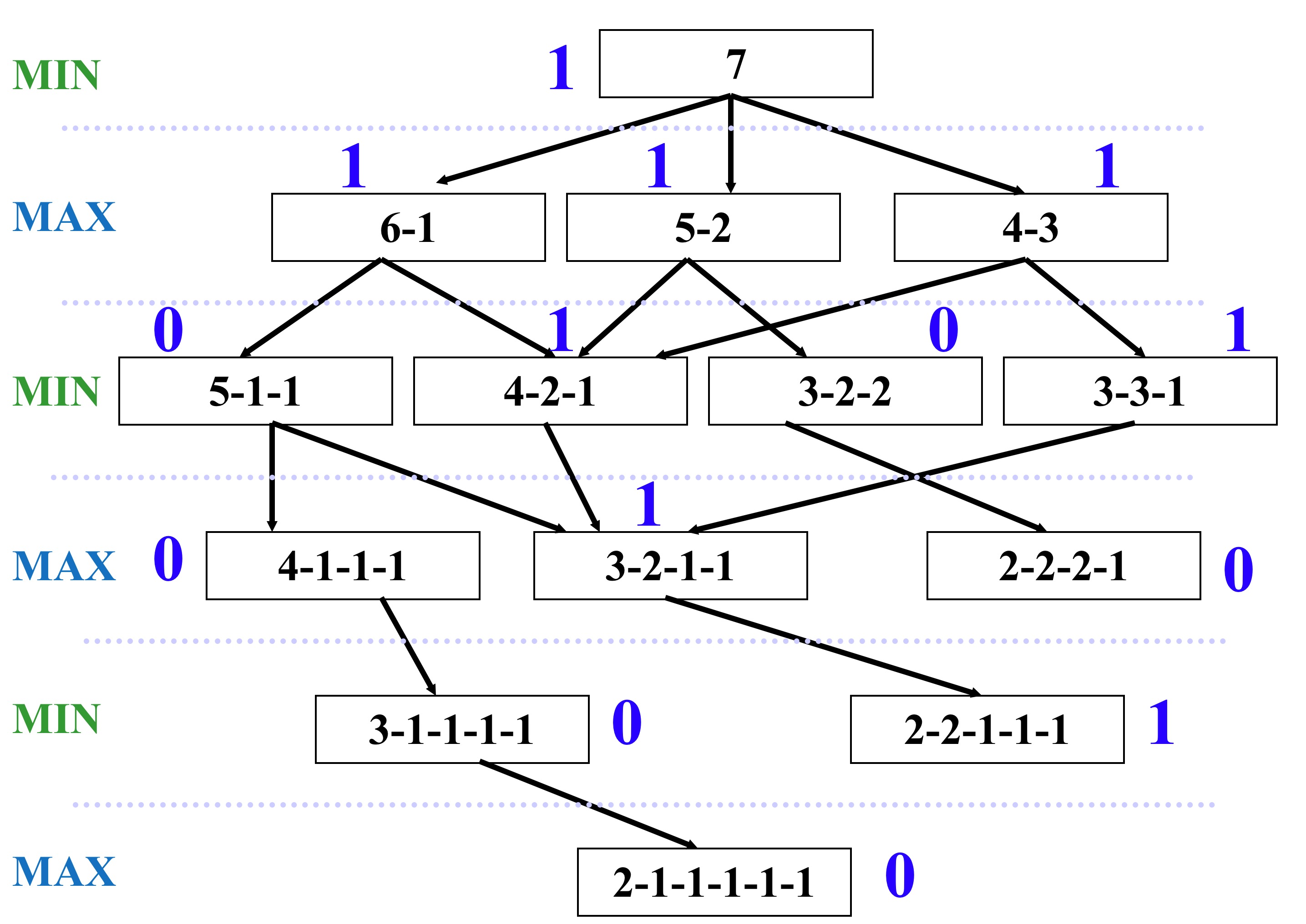
4.2.6.7 Minimax
Minimax: a decision rule for minimizing the possible loss for a worst case scenario.
(to solve zero-sum games that can be described by a game tree.)
Minimax Value: the smallest value that the other players can force the player to receive. If a player adopts the minimax strategy, the minimax value can be guaranteed no matter what strategies other players adopt.
https://youtu.be/zp3VMe0Jpf8
4.2.7 Evolutionary Game Theory (EGT)
4.2.7.1 Problems with Classical Game Theory
Assumption of rationality: not always appropriate
Limitation of Nash equilibrium: maybe too many Nash equilibria
Difficulty in computing Nash equilibrium: NP hard
4.2.7.2 Some Basic Concepts
Darwinian evolution is based on three fundamental principles: reproduction, mutation and selection.
Evolutionary Game Theory (EGT) is the application of game theory to evolving populations.
An evolutionary version of game theory does not require players to act rationally – only that they have a strategy.
It focus on the dynamics of strategy change in the population.
Invasion: mutations that successfully out-compete the current genotypes and increase in number
Evolutionarily Stable Strategy (ESS): is a strategy which, if adopted by a population in a given environment, cannot be invaded by any alternative strategy that is initially rare.
4.2.7.3 Models of EGT
EGT encompasses Darwinian evolution, including competition (the game), natural selection (replicator dynamics), and heredity.
Components:
Population
Game
Replicator Dynamics
Phases:
The model (as evolution itself) deals with a Population (Pn). The population will exhibit Variation among Competing individuals. In the model this competition is represented by the Game.
The Game tests the strategies of the individuals under the “rules of the game”. These rules produce different payoffs – in units of Fitness (the production rate of offspring). The contesting individuals meet in pairwise contests with others, normally in a highly mixed distribution of the population. The mix of strategies in the population affects the payoff results by altering the odds that any individual may meet up in contests with various strategies. The individuals leave the game pairwise contest with a resulting fitness determined by the contest outcome, represented in a Payoff Matrix.
Based on this resulting fitness each member of the population then undergoes replication or culling determined by the exact mathematics of the Replicator Dynamics Process. This overall process then produces a New Generation P(n+1). Each surviving individual now has a new fitness level determined by the game result.
The new generation then takes the place of the previous one and the cycle repeats. The population mix may converge to an Evolutionary Stable State that cannot be invaded by any mutant strategy.
4.2.7.4 Replicator Dynamics
Replicator Equation: a deterministic monotone non-linear and non-innovative game dynamic used in evolutionary game theory.
where:
xi is the proportion of type i in the population
x = (x1, ..., xn) is the vector of the distribution of types in the population
fi(x) is the fitness of type i (which is dependent on the population)
φ(x) is the average population fitness (given by the weighted average of the fitness of the n types in the population)
Evolutionarily Stable State: population's genetic composition is restored by selection after a disturbance, provided the disturbance is not too large. Such a population can be genetically monomorphic or polymorphic.
Evolutionarily Stable Strategy (ESS): a strategy which, if adopted by a population in a given environment, cannot be invaded by any alternative strategy that is initially rare.
ESS = Nash Equilibrium + Stability Condition
E(S, T): the payoff for palying strategy S against stategy T
If S is an ESS, then for all T ≠ S
E(S, S) ≥ E(T, S) and E(S, T) > E(T, T)
Some facts:
ESSes and Nash equilibria often coincide.
Every ESS corresponds to a Nash equilibrium, but some Nash equilibria are not ESSes.
Some games have ESS, some don’t have.
Example: The Prisoners Dilemma
Payoff:
T>R>P>S, 2R>T+S
=> Defect is an ESS (and the only Nash equilibrium in this game)
2 genotypes in the population
Cooperators (C-types): always cooperate
Defectors (D-types): always defect
(Suppose that the proportions of cooperators and defectors in the population are initially x and 1-x respectively)
Expected Utility:
A cooperator meets another cooperator with probability x and a defector with probability 1-x and expects to earn: F(c) = x(3) + (1-x)(0)
A defector will also meet a cooperator with probability x and a defector with probability 1-x and expects to earn: F(d) = x(5) + (1-x)(1)
Selection:
The cooperators will outbreed the defectors if:
F(C) > F(D)
=> x(3) + (1-x)(0) > x(5) + (1-x)(1)
=> x < - 1
=> cannot hold
=> So the cooperators will die out
=> 100% defectors is an Evolutionary Stable State.
Example: The Hawk-Dove Game (The Game of Chicken)
The Game of Chicken: while it is to both players’ benefit if one player yields, the other player's optimal choice depends on what his opponent is doing: if his opponent yields, the player should not, but if the opponent fails to yield, the player should.
Payoff:
V: value of the contested resource
C: the cost of an escalated fight
=> No strategy is an ESS.
(There are two Nash equilibria in this game: Hawk-Dove and Dove-Hawk.)
It is (almost always) assumed that the value of the resource is less than the cost of a fight, i.e., C > V > 0. If C ≤ V, the resulting game is not a game of Chicken but is instead a Prisoner's Dilemma.
2 genotypes in the population
Hawk: always fight
Dove: share or concede
(Suppose that the proportions of Hawks and Doves in the population are initially x and 1-x respectively.)
Expected Utility:
A Hawk meets another Hawk with probability x and a Dove with probability 1-x and expects to earn: F(H) = x(V-C)/2 + (1-x)(V)
A Dove will also meet a Hawk with probability x and a Dove with probability 1-x and expects to earn: F(D) = x(0) + (1-x)(V/2)
Selection:
The Hawks will outperform the Doves if:
F(H) > F(D)
=> x(V-C)/2 + (1-x)(V) > (1-x)(V/2)
=> x < V/C
The Doves will outperform the Hawks if:
x > V/C
The Doves and the Hawks will be in balance if:
x = V/C
Analysis:
C>V>0. Otherwise the Hawks will dominate.
x = V/C is an equilibrium state, in which the fitness of the Hawks and the Doves is the same and the percentages of two genotypes remain stable.
When C >> V, the percentage of the Hawks will be at low level in the population because fighting is expensive.
When C -> V, the percentage of the Hawks will be at high level in the population because fighting is cheap.
Example: The Iterated Prisoner's Dilemma (IPD)
The Iterated Prisoner's Dilemma (IPD): two players play prisoner's dilemma more than once in succession and they remember previous actions of their opponent and change their strategy accordingly
No ESS =>
Oscillation
Converge to a stable state (depends on initial population and mutation rate)
Divergence
Strategies:
Always Defect (AllD)
Always Cooperate (AllC)
Tit-for-tat (TFT): If you cooperated, I cooperate; If you defected, I defect.
Tit-for-two-tat (TFTT)
Gram trigger (Revenge)
Win-stay, lose-shift
Random
...
5 Bayes Fundamental
5.1 Some Basic Concepts
Bayesian Probability: a formalism that allows us to reason about beliefs under conditions of uncertainty.
P(A): the probability P of an uncertain event A
P(a|K): represents a belief measure
(e.g. a person's subjective belief in a statement a will depend on some body of knowledge K)
when K remains constant we just write P(a) in simplification.
Bayes Rule:
Prior Probability (Prior) of an uncertain quantity: the probability distribution that would express one's beliefs about this quantity before some evidence(data) is taken into account.
Posterior Probability: is the probability of assigning observations to groups given the data. (i.e. the conditional probability that is assigned after the relevant evidence or background is taken into account.)
In general, we want to relate an event (E) to a hypothesis (H) and the probability of E given H.
5.2 Bayes’ theorem
6 Machine Learning & Data Mining
6.1 Machine Learning
6.1.1 What
Machine Learning: relates with the study, design and development of the algorithms that give computers the capability to learn without being explicitly programmed.
An agent is learning if it improves its performance on future tasks after making observations about the world.
6.1.2 Why
The designers cannot anticipate all possible situations that the agent might find itself in.
The designers cannot anticipate all changes over time.
Sometimes human programmers have no idea how to program a solution themselves.
6.2 Supervised Learning
6.2.1 What
Supervised Learning: the agent observes some example input- output pairs and learns a function that maps from input to output
6.2.2 How
given input samples (x) and labeled outputs (y) of a function y = f(x), “learn” f, and evaluate it on new data
Classification: y is discrete (class labels). Learn a decision boundary that separates one class from another
Regression: y is continuous, e.g. linear regression. Learn a continuous input-output mapping, also known as “curve fitting” and “function approximation”
given only samples x of the data, infers a function f such that y = f(x) describes the hidden structure of the unlabeled data - more of an exploratory/descriptive data analysis
Clustering: y is discrete. Learn any intrinsic structure that is present in the data
Dimensional Reduction: y is continuous. Discover a lower- dimensional surface on which the data lives
Data Mining: the exploration and analysis of large quantities of data in order to discover valid, novel, potentially useful, and ultimately understandable patterns in data.
Valid: hold on new data with some certainty
Novel: non-obvious to the system
Useful: should be possible to act on the item
Understandable: humans should be able to interpret the pattern
Machine Learning vs Data Mining
Machine learning: predicts with models
Data mining: explains patterns
Process of KDD
The knowledge discovery in databases (KDD) process is commonly defined with the stages:
use historical data to build models of fraudulent behavior
use data mining to help identify similar instances
Customer relationship management (CRM)
Which of my customers are likely the most loyal
Which are most likely to leave for a competitor
Identify likely responders to sales promotions
Scienctific viewpoint:
Medicine: disease outcome, effectiveness of treatments
analyze patient disease history & find relationship between diseases
Astronomy: scientific data analysis
identify new galaxies by the stages of formation
Web site design and promotion
find affinity of visitor to pages and modify layout
6.5.3 Tasks
Data mining involves six common classes of tasks:
Anomaly detection (outlier/change/deviation detection) – The identification of unusual data records, that might be interesting or data errors that require further investigation.
Association rule learning (dependency modelling) – Searches for relationships between variables. For example, a supermarket might gather data on customer purchasing habits. Using association rule learning, the supermarket can determine which products are frequently bought together and use this information for marketing purposes. This is sometimes referred to as market basket analysis.
Clustering – is the task of discovering groups and structures in the data that are in some way or another "similar", without using known structures in the data.
Classification – is the task of generalizing known structure to apply to new data. For example, an e-mail program might attempt to classify an e-mail as "legitimate" or as "spam".
Regression – attempts to find a function which models the data with the least error that is, for estimating the relationships among data or datasets.
Summarization – providing a more compact representation of the data set, including visualization and report generation.
In this module:
Classification: Identify to which set a new observation belongs
Clustering: Group a set of objects so objects in the same cluster are more similar
Association rule discovery: Discover interesting relations between variables in large databases ØIdentify rules using some measures
Classification: learn a method to predict the instance class from pre-labeled (classified) instances
Many approaches:
Regression
y = ax1 + bx2 + c
Decision Trees
divide decision space into piecewise constant regions
Neural Networks
partition by non-linear boundaries
Support vector machines
...
Application:
For target marketing: reduce cost of mailing by targeting consumers who are likely to buy a
new cell-phone product.
6.5.3.1.1 Approach 1: Regression
To find the best line (linear function y=f(x)) to explain the data.
Cons:
Not flexible enough
6.5.3.1.2 Approach 2: Decision Tress
Nodes:
Internal node: decision rule on one or more attributes
Leaf node: a predicted class label
Pros:
Reasonable training time
Can handle large number of attributes
Easy to implement
East to interpret
Cons:
Simple decision boundaries
Problems with lots of missing data
Cannot handle complicated relationship between
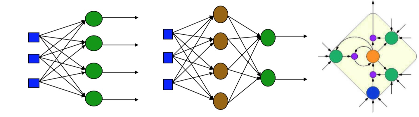
6.5.3.1.2 Approach 3: Neural Networks
Pros:
Can learn more complicated class boundaries
Can be more accurate
Can handle large number of features
Cons:
Hard to implement: trial and error for choosing parameters and network structure
Slow training time
Can over-fit the data: find patterns in random noise
Hard to interpret
6.5.3.2 Task 2: Clustering (Unsupervised Learing)
Clustering: partition the data so the instances are grouped in similar items by using distance/similarity measure.
A set of data points, each with a set of attributes and a similarity measure, find clusters such that
Data points in one cluster are more similar
Data points in separate clusters are less similar to one another
Methods of similarity measure:
Euclidean or Manhattan distance
Hamming distance
Other problem specific measures
Approches:
Partitioning-based clustering
K-means clustering
K-medoids clustering
Density-based clustering
Separate regions of dense points by sparser regions of relatively low density
Application:
For market segmentation: divide a market into distinct subsets of customers, any subset may be a market target
6.5.3.2.1 Partitioning-Based Clustering: K-Means
Goal: minimise sum of square of distance
Between each point and centers of the cluster
Between each pair of points in the cluster
Algorithm:
Initialize K cluster centers
random, first K, K separated points
Repeat until stabilization:
Assign each point to closest cluster center
Generate new cluster centers
Adjust clusters by merging or splitting
6.5.3.2.2 Density-Based Clustering
Cluster: a connected dense component
Density: the number of neighbors of a point
6.5.3.3 Task 3: Association Rule Discovery
Associate Rule Discovery: discover interesting relations between variables in large databases.
Associate Rule: discover dependency rules, which predict occurrence of an item based on occurrences of other items.
Application:
market basket analysis:
Association rules: 60% of customers who purchase X and Y also buy Z
Sequential patterns: 40% of customers who first buy X also purchase Y within three weeks
7 (Artificial) Neural Networks
7.1 Neural Networks
7.1.1 What
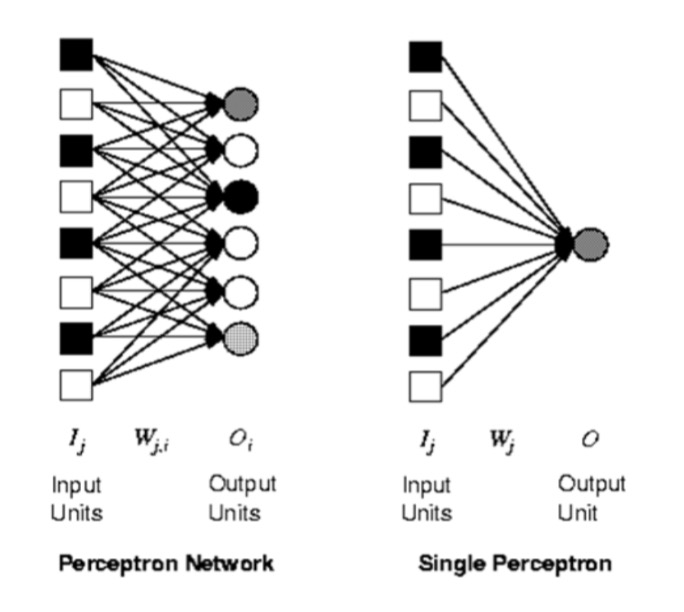
Artificial neural networks (ANNs) or connectionist systems are computing systems vaguely inspired by the biological neural networks that constitute animal brains.
Consists of:
A set of inputs - (dendrites)
A set of resistances/weights – (synapses)
A processing element - (neuron)
A single output - (axon)
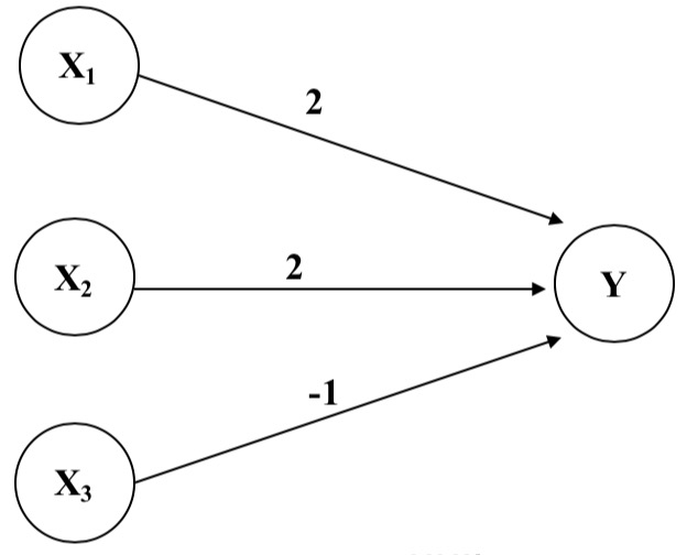
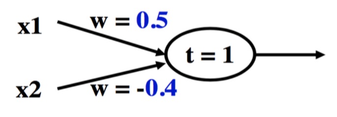
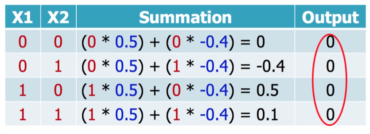
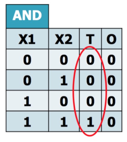
7.1.2 The First Neural Networks
y_in = x1 * 2 + x2 * 2 + x3 * (-1)
For the network shown here the activation function for unit Y is